Linear Programming Solutions
It is easy to understand how linear programming works by considering a problem with only two decision variables. Of course this is a trivial problem, but only problems of this size can be easily drawn! The problem is:
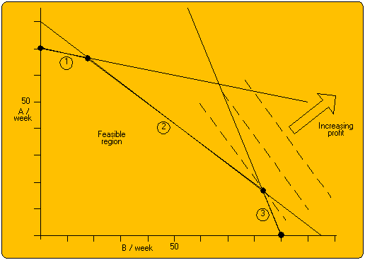
A small factory manufactures two types of chair legs (A and B). Each type of chair leg requires turning on a lathe, planing and polishing. The company has one lathe, one planing machine and one polishing machine, each running for 37 hours (2200 minutes) per week. For products A and B it takes 31 and 6 minutes on the lathe, 27 and 20 minutes for planing and 10 and 24 minutes for polishing. The company makes a profit of Ł3.00 per A chair leg and Ł4.50 per B chair leg. How many chair legs of each type should the company make to maximise its profit? The graphical solution to this problem is shown below.

The constraints on the working minutes for turning, planing and polishing are given by lines with 1, 2 and 3 in circles. Together with the A and B axis these demarcate a feasible region (for any point in this region it is possible to make the numbers of A and B items within a week).
The profit is 3*A+4.5*B which forms the family of dashed lines. The maximum profit obtainable occurs when one of these lines just touches the feasible region. This will always occur at a vertex of the feasible region (in rare cases the optimum may include 2 adjacent vertices and the line between them). The vertices of the feasible region are marked by black dots, the optimum vertex has a circle around it. For this problem the company should make 83 B items and 17 A items. With this work schedule planing and polishing are fully loaded, but the lathe will have spare capacity.
If the profit for B items increases the gradient of the cost lines will increase and eventually the optimum will be the vertex on the B axis. Conversely if the profit for A items is increased then eventually the optimum would be the vertex with about 20 B items. Whatever the profits for the items are the optimum will always be at one of the four vertices.
The Simplex algorithm would start at a feasible vertex (in this case the origin) then move along an edge of the feasible region that increases the profit until it meets the next vertex. At the next vertex it would check the edges and again move along an edge that increases the profit. If no edge increases the profit then the optimum must have been found. For the current problem the Simplex algorithm would start at the origin and move along the B axis to the vertex at B=90. It would then move along edge 3 until it reached the next vertex, which in this problem is the optimum. At the optimum no edge increases the profit. The Simplex algorithm always works for a constrained non-empty feasible region because the feasible region is convex so that there are no local minima. The Simplex algorithm can solve LP problems with hundreds of decision variables.
Optimal Solutions welcomes enquiries on Linear Programming, and would be pleased to offer consultancy on this, or any other aspect of Optimisation. You can get in touch by sending a message from our Contact Us page, or by calling us on the number below.